Do Digital Monkeys Dream of Electronic Sonnets?
The curious birth of information from randomness
What is Information?
We encounter information in various forms, such as data entries on an Excel sheet, news reports, or social media posts. This information can be straightforward or intricate, based on facts or personal opinions, and can be either true or false. Information is the currency we use to exchange knowledge, and as the saying goes, knowledge is power. The information serves as the raw material that powers our understanding.
What is the mathematical value of information?
Information theory is a field of applied mathematics that focuses on how we measure, store, and communicate information.
This standard was not decided haphazardly. The binary values of 1 and 0 could be used to represent simple logical operations, and it is this versatility that allowed computers to tackle a wide array of problems
In the fields of physics and cosmology, information has become a crucial tool to explore the underlying principles of the universe.
The Infinitely Small Possibilities
The infinite monkey theorem is a popular thought experiment that shows the reality of minuscule probabilities. It considers the possibility that if you had a monkey use a typewriter, and the monkey could hit random keys for an infinite amount of time, that eventually he would create a perfect copy of William Shakespeare’s complete works.

For now, infinity remains a mathematical concept, far removed from the reality of physics.
In the US Powerball, five balls are chosen at random from a pool of 69 numbered balls. Additionally, one red Powerball is chosen from a set of 26 numbered balls. If you correctly guess some of the numbers, you can win a portion of the prize money. However, you need to guess all the numbers in the correct order to win the grand prize.
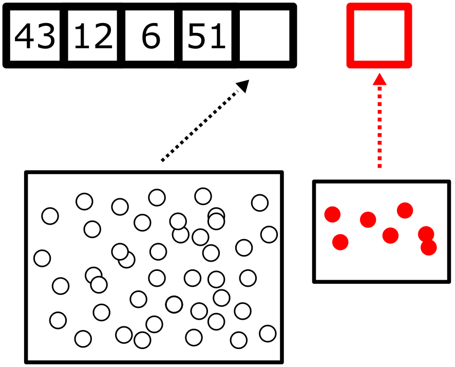
How likely are you to win the jackpot? First, let’s consider the total number of possible combinations that might occur in this game. Combinatorics is a branch of mathematics that deals with the study of counting and arranging objects or elements. In this case, we only care about how many different \(r\) arrangements we can get from \(n\). When \(r = 5\) and \(n = 69\) the solution is as follows:
\[C(r,n) = \frac{n!}{r!(n-r)!} = \frac{69!}{5!(69-5)!} = \frac{69 \times 68 \times 67 ... \times 1}{5 \times 4 ... \times 1 \times 64 \times 63 ... \times 1} = 11,238,513\]For the single red Powerball, it is as simple as:
\[C(r,n) = \frac{n!}{r!(n-r)!} = \frac{26!}{1!(26-1)!} = \frac{26 \times 25!}{1 \times 25!} = 26\]So we are left to choose between \(11,238,513\) (known as \(N\)) possible combinations of numbers for the white balls, and 26 different numbers for the red Powerball. To win the grand prize we need to determine one single combination of both. What is the probability that we do this? This ends up being a simple calculation since we know that there is only 1 (or \(n\)) possible combination that ends up being the winning attempt:
\[P = \frac{n}{N} = \frac{1}{11,238,513} \times \frac{1}{26} = \frac{1}{292,201,328}\] Do I feel lucky
To calculate the probability of success for the infinite monkey theorem, we need to consider more than just the 26 letters of the English alphabet. We assume that the monkey has access to a keyboard that includes uppercase and lowercase letters, numbers, punctuation symbols, and other symbols necessary for a book (such as spaces and new lines). Altogether, this gives us about 88 inputs to work with.
\[P = \frac{n}{N} = \frac{1}{88} = 0.0113636... \approx 1.14\%\]The Gutenberg project is a repository that provides an extensive source of books that have way past expired their copyright rights. Using this resource we can acquire a copy of William Shakespeare’s complete works in .txt format. The number of characters in “The Complete Works of William Shakespeare” is about 5,480,868. For the monkey to write the full text in a single sitting becomes vanishingly small:
\[P(n, N) = \frac{n}{N} = (\frac{1}{72})^{5,480,868} = 10^{-10^{7.007739000088917}}\]This probability increases on every attempt. This implies that the event eventually happens, just that no one would be alive to confirm it:
\[P_{\notin}(x) = (1 - P)^{x}\] \[P(x) = 1 - (1 - P_i)^{x} \approx 1\] \[P(x) = 1 - (1 - 10^{-10^{7.007739000088917}})^{x} \approx 1\]Down to Monkey Business
The infinite monkey theorem proposes the idea that unlikely events can occur. This concept has been the subject of many simulations and studies that try to replicate this phenomenon.
To build our simulation, we will use computers that will act as digital counterparts to our monkeys. This way, we can accelerate the typing process by having the computer do the same work of multiple monkeys in tandem. Additionally, we need to specify the way that our ‘digital monkeys’ will output data. To get closer to theory, we also need to recreate the method in which monkeys would input characters. For this purpose, I chose the reliable 1973 IBM Selectric 721, as it contains all the letters and symbols that they would need.
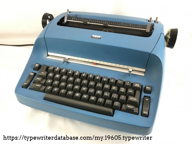
To represent each keystroke in our simulation, we will generate a random binary number that will indicate an input. A 7-bit binary number gives us enough combinations to represent every character on the Selectric typewriter. Binary numbers have the advantage of being easy to quantify in terms of digital size. Using a typical encoding like ASCII or UTF-8, each character has a size of one byte. This means that each input to the typewriter has a size of 7 bytes (one byte per bit), and each output from the typewriter (representing a keystroke) has a size of 1 byte. To generate truly random inputs, we use the libsodium library to create cryptographically secure random bytes.
Now that we have our tools, let’s start defining our workspace. Until the machines rise against us, we can use any different number of ‘digital monkeys’ for any amount of time. Unfortunately, we still have to consider the computational cost that would allow our computer to do the work. Google Colab is a free, cloud-based platform for running and sharing code. Although predominantly used to run Python scripts, we can use the instances provided by Colab as a computer that runs processes in the cloud. These cloud computers, like any computer, have a limit on what they can do simultaneously. Additionally, since this is a dynamic environment (resources are dependent on the number of users using the service), we cannot easily know the number of monkeys that we can assign to this task. We can try to get an estimate of the optimal number of ‘digital monkeys’ that we can have working in parallelism. To do so, we can set a loop that increases the number of processes for a directly proportional set of time, and then look at the average time it takes for the process to finish.
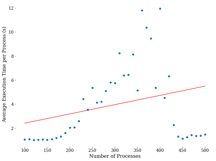
At low levels of parallelism (e.g. 100 processes), the program may be able to efficiently utilize the available hardware resources without encountering bottlenecks or fighting for shared resources. At high levels of parallelism (e.g. 500 processes), the program may start to encounter hardware limitations such as network bandwidth, disk I/O, or memory bandwidth that limit the overall performance of the program. Not a great look at how well-optimized this simulation is, but good enough to get the data that we need. We will use 120 for our number of processes as this is the minimum value in our line of best fit.
In order to determine how many words we produce we need to use a dictionary. This is not your typical dictionary, as we do not require any definitions in this simulation.
All the World’s a Monkey’s Stage
At the end of our simulation, we managed to produce 3.7 Gbs of text in 156 hours with the help of our 120 digital monkeys. So what does this look like? Let’s examine the overall dataset:
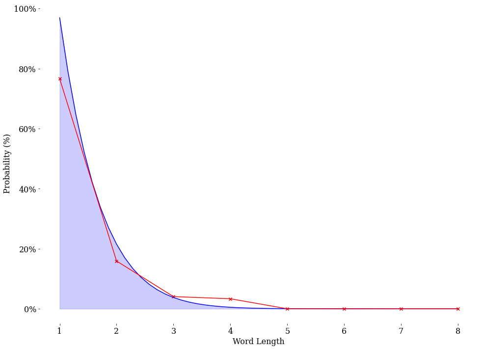
This simply won’t do. We are currently including every single character in the data, regardless if it is significant or not. We need to establish criteria for tagging words in our dataset. Although the letter ‘a’ is a perfectly reasonable word, it leaves too much to interpretation regarding how much ‘information’ it provides in the text. We can’t be sure of what is a random input or what would be a significant word. So for this analysis, we will simply ignore any words that are made of a single character.
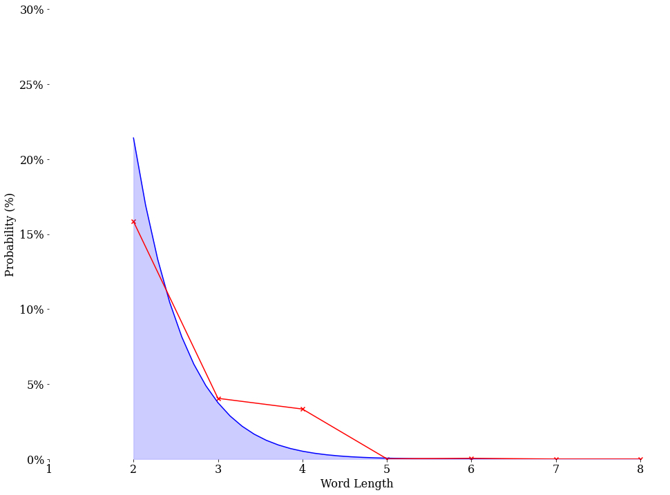
Our analysis shows that there is a \(15.915\)% chance that a two-letter word shows up in our dataset, and that every additional character decreases the likelihood significantly as the word length increases. It is always wise to make sure that our results make sense. What is the expected length of words in our dataset when we analyze the distribution of word lengths in our dictionary?
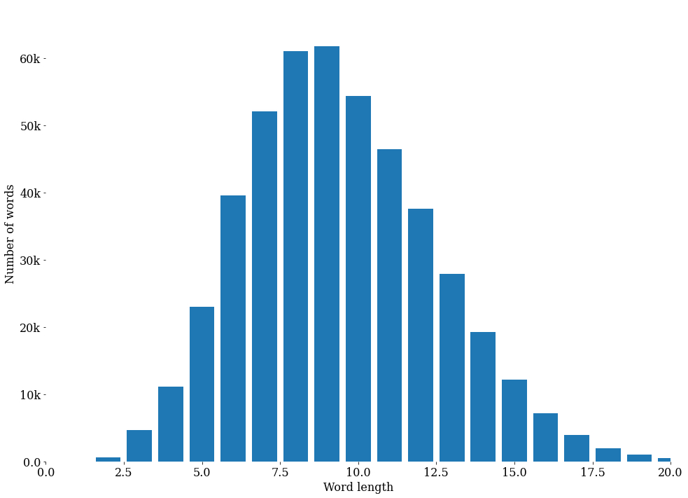
Based on this graph alone, it might be logical to think that ~\(10\) letter words should be more prevalent in our data. To resolve this inconsistency, we must return to our probability calculations. We must remember that every consecutive character is confined by a probability. If we want a \(6\) letter word and we currently have \(88\) different options, then every input to our data is restricted by the distribution of this probability:
\[(\frac{1}{88})^{6} = \frac{1}{88} \times \frac{1}{88} \times ... \times \frac{1}{88} = \frac{1}{464,404,086,784}\]Now that we have the probabilities in place, how does it help us determine the amount of information contained? Information theory provides us with a method to quantify the amount of information contained in a file using the concept of entropy. The mere mention of entropy can cause anxiety to most scientists. It is a complex and abstract concept that is central to several fields of science. It has multiple meanings, different interpretations, and a wide array of formulations. More than anything, people find it non-intuitive. In this case, entropy measures the amount of uncertainty or randomness in our data.

A file contains more information if the data is more unpredictable, according to the fundamental principle of using entropy to quantify information. So entropy can become our measurement of how much information there is in a file. Information entropy is calculated by identifying all possible outcomes or symbols that can appear in a file. Symbols may include individual characters in a text file or individual bits in a binary file, among other possibilities. The entropy of information can be calculated using the following formula:
\[H(p_i) = -Σ \enspace p_i \enspace log_2 \space p_i\]Where \(H\) is the entropy of information, \(p_i\) is the probability of symbol \(i\) occurring, and \(log_2\) is the base-2 logarithm.
Let’s consider the entropy of information for “The Complete Works of William Shakespeare” first. After filtering out all the copyright and index contents, we are left with 959,976 words.
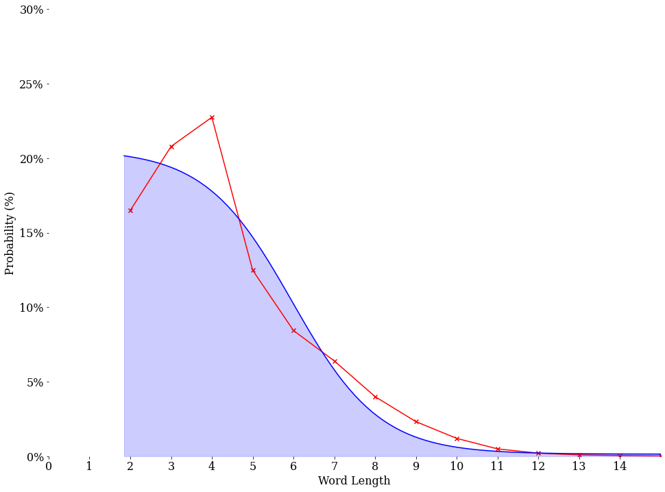
Calculating the entropy requires us to define a probability distribution that a word of a particular length would be found in the file:
\[p_i = \frac{\text{Number of instances}}{\text{Total number of words}}\] \[\qquad\] \[H(p_i) = -Σ \enspace p_i \enspace log_2 \space p_i = 2.839 \text{bits}\]Performing the same calculation to our simulation data we get that the entropy of information based on word length is \(1.242\) bits, which is quite strange. Why would we get a lower entropy when the creation of this data has been completely random? The definition of entropy should be the amount of randomness in our data. The entropy we got from our simulation is not a mistake. Claude Shannon calculated the conditional entropy of an English text based on letter frequencies, but the method can be adapted to word frequencies as well. Shannon found that the entropy per letter of English text was about \(2.3\) bits.
Keep in mind, we’re not dealing with a random sequence of words in Shakespeare’s writings. Sentences have a predefined structure that goes beyond simple grammatical rules. Sometimes you can even predict a statement before it _____.

The online game Wordle became a massive hit in the year 2021. It challenges a player to guess a five-letter word in six attempts and reveals feedback on which letters are correct, incorrect, or in the correct position. Naturally, we start by choosing a word that eliminates a significant number of vowels or maybe very common consonants. With the given feedback, we can correctly guess our words in as little as two attempts.
Introducing Random-le, a game that challenges you to guess a random five-character ‘string’ in six attempts. Not impossible, but not something I’ll be winning or even attempting at all.
What if we were to be more strict regarding our analysis? If we were to imitate more closely the rules of language, then the entropy in our analysis should resemble those found in standard texts. To illustrate how a more meticulous analysis should lead us closer to Shannon’s results, let’s do one final calculation. We did not consider the effect that cases would have on the readability of the file. Meaning that so far, ‘Hello World’ and ‘helLo wORlD’ are the same. To rectify this, let’s consider ‘penalizing’ the word count for every mistake in the word. Meaning that ‘enTRopy’ would be counted as a \(5\) letter word instead of \(7\). For example, the probability of finding a two-letter word is now \(12.227\)% instead of the previous \(15.915\)%. By applying additional rules, we’ve increased the entropy of information based on word length to \(1.328\) bits. Which inches us closer to the entropy found in Shannon’s work and Shakespeare’s writings.
Where art thou my Entropy?
Originally, the word “entropy” was coined by German physicist Rudolf Clausius in 1865.
This measurement helps us understand the disorder or randomness of a system, and it increases as the system becomes more disordered. Imagine a box of magic bouncing balls. They’re magical in the way that they never lose their momentum. Meaning that once they start bouncing, they can’t stop unless we manually set them in stasis. Likewise, they won’t be able to start moving without our intervention. We start with every ball perfectly at rest. We would always be able to easily determine each ball’s position and velocity (x, 0). Our box contains no uncertainty, no randomness, and no entropy.
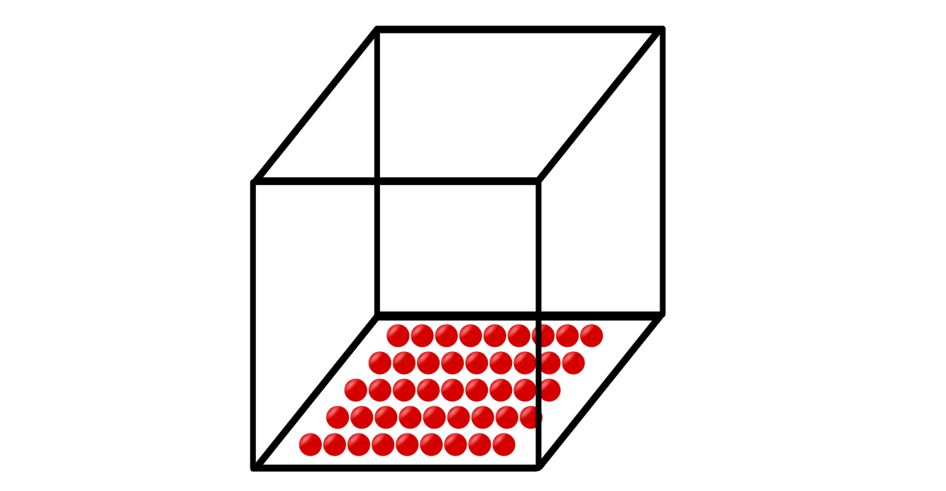
If we were to set one of our balls in motion, then we end up increasing the entropy of the box slightly. Now it’s going to be more challenging to define the position and velocity of every ball. We’ve added some uncertainty to our system. The same occurs by putting every ball in our box in motion. The entropy rises directly by increasing the number of balls and their speed. This same concept can be applied to a system with gas. Where every bouncing ball can be replaced with a molecule. The entropy in this system can be calculated, and from that, properties such as temperature and pressure can be naturally inferred.
Is Shannon’s entropy of information the same as this? Entropy in statistical mechanics and information theory are both measures of disorder or uncertainty, and they both have the same mathematical form when expressed in terms of probabilities. The Boltzmann distribution is a probability distribution that gives the probability of a system being in a certain state as a function of that state’s energy and the temperature of the system.
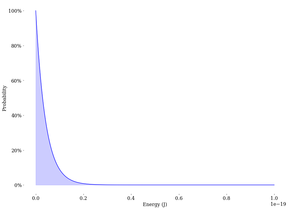
Energy and information are both subject to the same fundamental constraints of thermodynamics, and they can be seen as two different forms of entropy. There is a connection between bits of information and bits of energy, where the energy content of a physical system is related to the amount of information that it can store or process. The entropy of a black hole can be thought of as the amount of information that is hidden behind the event horizon, beyond the reach of any observer outside the black hole. The energy of a black hole can be converted into information, or vice versa, through the process of Hawking radiation.

You might be wondering the difference between these ‘bits’ from entropy and the ‘bits’ encoded in the 3.7 Gbs of data we have generated.
Tomorrow and tomorrow and tomorrow
Creeps in this petty pace from day to day
To the last syllable of recorded time,
And all our yesterdays have lighted fools
The way to dusty death. Out, out, brief candle!
Life’s but a walking shadow, a poor player
That struts and frets his hour upon the stage
And then is heard no more. It is a tale
Told by an idiot, full of sound and fury,
Signifying nothingIn many theatre groups, the implication of redundancy might earn you a beating.
By this measure, a highly compressed cat video contains an entropy much larger than its file size. This video would have very little redundancy in its data. But the significance of the information in The Bard’s work is inherently more valuable.
Struggling with the concept of entropy might as well be added as one of the laws of physics. But its importance is so profound that it incites a desire to learn more about it. The results of this simulation should show you that the meaning of this physical property is much more complex than what Clausius and his contemporaries originally proposed. Hopefully reading this didn’t leave you too confused, but I also hope that it gave you the desire to understand more.
Infinite Monkey Simulation Python Notebook